How Sunny is Seattle?
A comparative look at solar resource availability

Is solar energy a viable resource for a city like Seattle?
My friend recently asked me this question.
I believe it's a fair question to ask. Seattle isn't known for its abundance of sunshine. As I write this post, it is a gloomy, cloudy and rainy day in Seattle. For those familiar with Seattle weather, this is not a surprise - fall and winter months are often cloudy and rainy.
In this post, we will answer this question by taking a look at the available solar resource for Seattle. We will also compare it against other cities - Boston, Austin and Berlin.
Note - this post is not a discussion on the differences in the local policies but only the resource availability.
Where do we get solar resource data?
National Renewable Energy Lab (NREL) provides access to the National Solar Radiation Database (NSRDB). NSRDB is collection of hourly and half-hourly values of meteorological data and solar radiation measurements.
We will download the data and perform the analysis using Python (You can also use the web interface to download the data, if you prefer).
To download the data programmatically, we will need a NREL Developer API key - it is free and the signup only requires your name and email (where you will receive the API key).
Installation
We will use a Python API that I have created, nrel-dev-api, to programmatically access data and analysis services from NREL. It currently covers all of the solar API endpoints that NREL provides, with future support for other services such as wind, electricity, etc.
python -m pip install --upgrade nrel-dev-api
Set your API key
from nrel_dev_api import set_nrel_api_key

set_nrel_api_key("YOUR_NREL_API_KEY")
Download NSRDB data
To download the data, we need the latitude and longitude for our city of interest as well as the year and time interval of our data. Seattle's latitude and longitude are 47.61 and -122.35, respectively.
First, we will check to see if there are any data available for the specified year, interval and location.
from nrel_dev_api.solar import (download_nsrdb_data,
                                get_nsrdb_download_links)

seattle_links = get_nsrdb_download_links(year=2016, interval=60, lat=47.61, lon=-122.35)
seattle_links
['https://developer.nrel.gov/api/nsrdb/v2/solar/psm3-download.csv?names=2016&wkt=POINT%28-122.35+47.61%29&interval=60&api_key=yourapikey&email=youremail']
The above get_nsrdb_download_links returns a list of available links for the location and year of interest. Once we have the links, we can pass them to download_nsrdb_data to download the data.
seattle_hourly_df = download_nsrdb_data(seattle_links[0], email="YOUR_EMAIL")
The download_nsrdb_data function returns a pandas dataframe containing hourly irradiance, temperature, humidity, pressure, etc. The specific value of interest to us here is the column named "GHI" which stands for 'Global Horizontal Irradiance'.
Global horizontal irradiance is the amount of irradiance falling on a surface that is horizontal to the surface of the earth. This value is of particular interest for solar installations.
We will first resample the "GHI" data monthly and then sum it up to create monthly global horizontal irrandiance data.
seattle_ghi_monthly_sum = 1e-3 * seattle_hourly_df["GHI"].resample("M").sum()
Note - the "GHI" data is in units of Wh/m2 and we are converting it to KWh/m2.
The resulting dataframe contains the monthly sum of "GHI" for the year 2016 in Seattle.
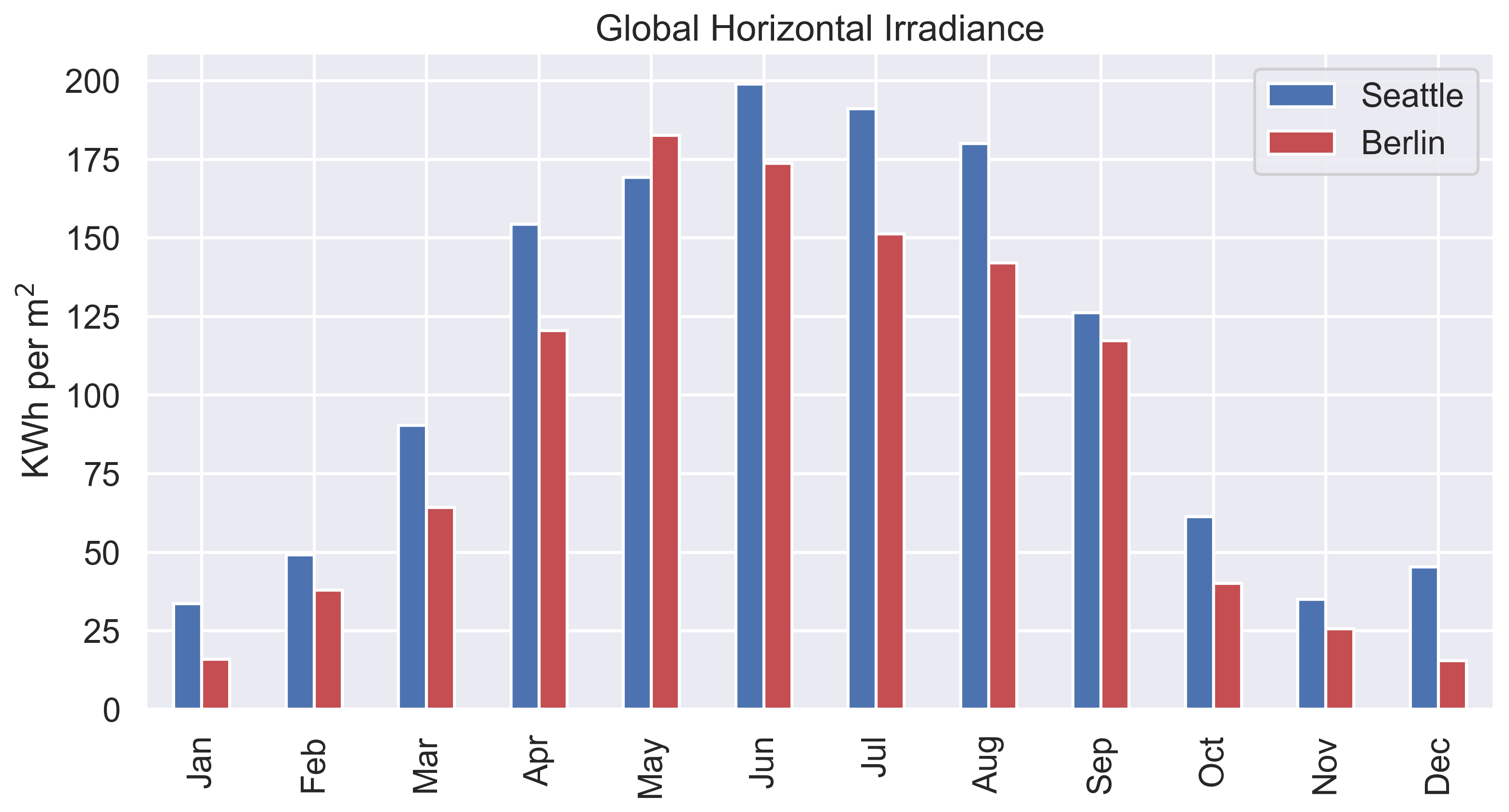
2016-01-31     33.661
2016-02-29     49.141
2016-03-31     90.370
2016-04-30    154.304
2016-05-31    169.188
2016-06-30    198.978
2016-07-31    191.013
2016-08-31    180.028
2016-09-30    126.233
2016-10-31     61.287
2016-11-30     35.059
2016-12-31     45.311
Freq: M, Name: GHI, dtype: float64
We can now repeat the process for Boston and Austin to get the monthly sum of "GHI" in 2016, boston_ghi_monthly_sum and austin_ghi_monthly_sum (If you want to see the code for Boston and Austin, check out the jupyter notebook).
Let's put all the monthly GHI data into a single dataframe.
import pandas as pd
import numpy as np

index = ["Jan", "Feb", "Mar", "Apr", "May", "Jun", "Jul", "Aug", "Sep", "Oct", "Nov", "Dec"]

ghi_df = pd.DataFrame(

    np.array([
        seattle_ghi_monthly_sum.values,
        boston_ghi_monthly_sum.values,
        austin_ghi_monthyl_sum.values
    ]).T,
    columns=["Seattle", "Boston", "Austin"],
    index=index
)
Finally, let's get GHI data for Berlin. NSRDB doesn't have data for Berlin but we can get it from PVGIS, a tool provided by the European Union science hub. After downloading the data, we can load it as a pandas dataframe.
berlin_monthly_df = (pd.read_csv("Monthlydata_52.516_13.377_SA_2016_2016.csv", sep="\t", skiprows=4, skipfooter=4)
                     .dropna(axis=1)
                     .rename(columns={"H(h)_m" : "monthly_ghi_kWh_m2"})
                    )

ghi_df["Berlin"] = berlin_monthly_df["monthly_ghi_kWh_m2"].values
	Seattle	Boston	Austin	Berlin
Jan	33.661	64.608	111.509	16.03
Feb	49.141	83.216	135.596	37.93
Mar	90.370	119.618	153.963	64.28
Apr	154.304	160.144	162.074	120.44
May	169.188	174.102	166.599	182.66
Jun	198.978	213.426	211.531	173.66
Jul	191.013	199.640	229.077	151.20
Aug	180.028	184.762	187.451	142.08
Sep	126.233	124.293	165.196	117.23
Oct	61.287	96.820	152.188	40.18
Nov	35.059	61.626	93.345	25.73
Dec	45.311	54.708	71.597	15.45
Let's visualize the differences in the irradiance data.
import seaborn as sns

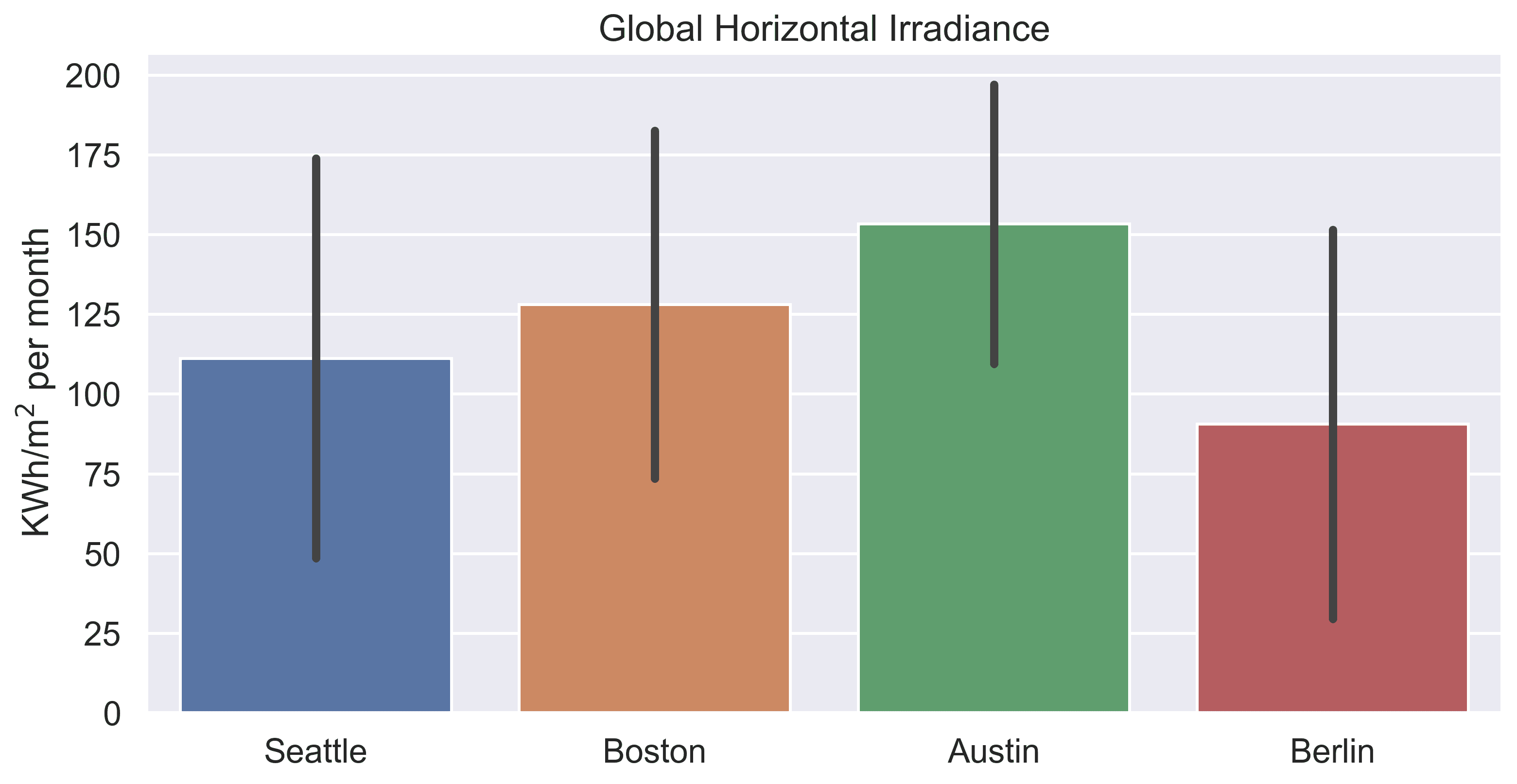
ax = sns.barplot(data=ghi_df, ci="sd")
ax.set_ylabel("KWh/m$^{2}$ per month")
ax.set_title("Global Horizontal Irradiance")

The barplot shows the average global horizontal irradiance per month (with errorbars representing the standard deviation) for the different cities in our dataframe.
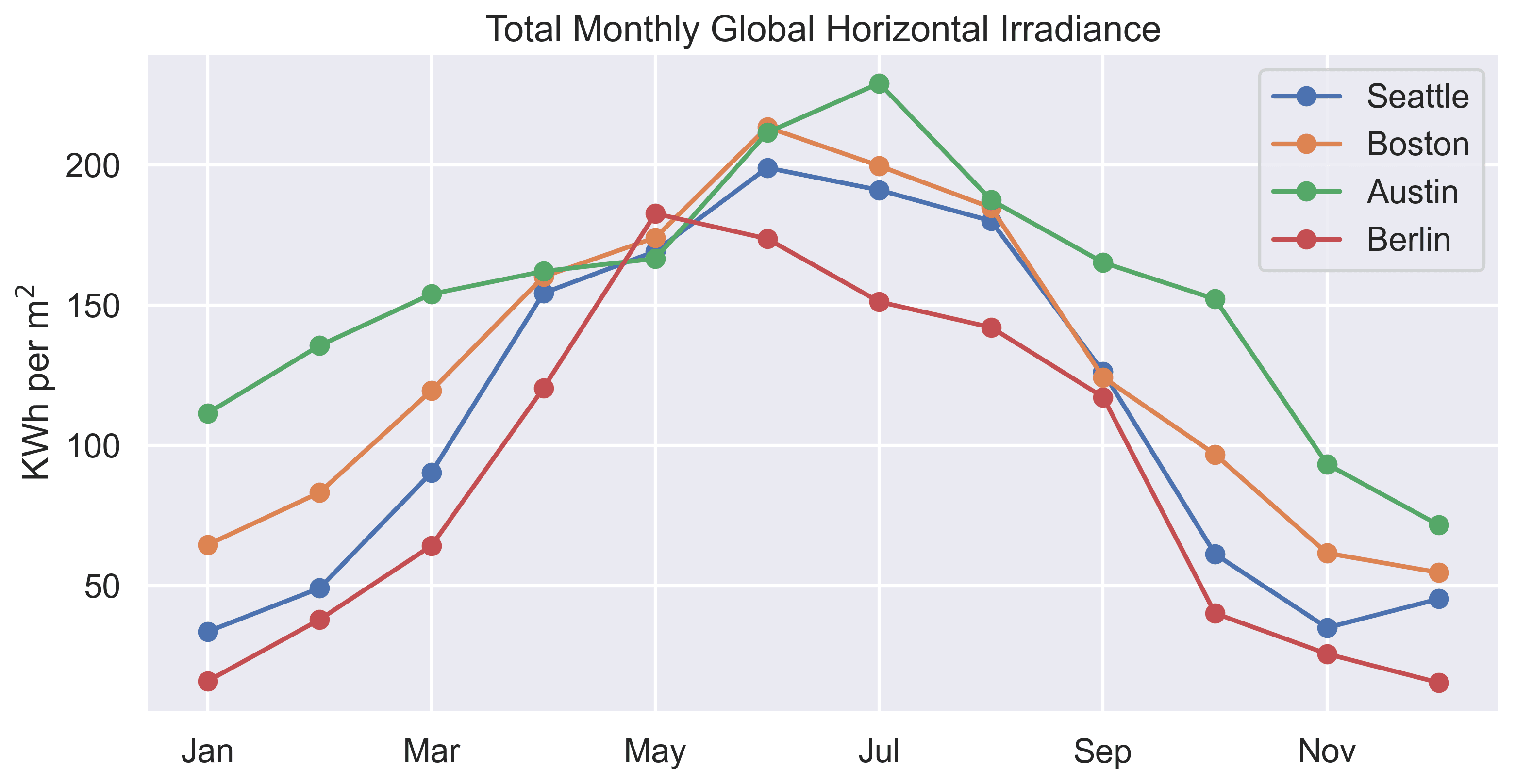
ax = ghi_df.plot(
    kind="line",
    ylabel="KWh per m$^{2}$",
    title="Total Monthly Global Horizontal Irradiance",
    style=["o-", "o-", "o-", "o-"]
)

The lineplot shows the monthly sum of global horizontal irradiance for the different cities in our dataframe.
# Annual Global Horizontal Irradiance
ghi_df.sum()  # KWh/m2
Seattle    1334.573
Boston     1536.963
Austin     1840.126
Berlin     1086.870
dtype: float64
Seattle gets sunlight comparable to Boston but lower than Austin, monthly as well as annually. The fall and winter months receive less sunlight, which is not surprising.

However, when we compare Seattle with Berlin, we see that Seattle gets higher solar irradiance thorughout the year. This is very promising for solar in Seattle (and Washington).
In 2020, Germany produced 51 TWh of electricity from solar despite getting less sun than Seattle! That's 10.5% of Germany's electricity generation.
Of course, there are differences in policies and cost of solar; but looking at the solar resource availability, there is no reason why solar energy can't be more successful in Seattle, Washington and the US in general.
Thanks for reading! You can find the notebook with the code here.